
¿Odias los anuncios? Ir Sin publicidad Hoy
La salida de EXPLAIN de SQL no tiene que parecer texto extraterrestre
Actualizado en
EXPLAIN muestra que la base de datos te está provocando. Aquí te explico cómo leer realmente los planes de consulta en PostgreSQL — los números de costo, los tipos de nodo y qué debes corregir.

ANUNCIO · ¿ELIMINAR?
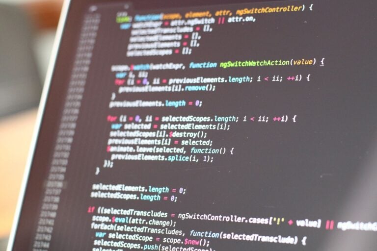
Tú ejecutas EXPLAIN en una consulta lenta. La base de datos te devuelve algo como esto:
Hash Join  (cost=145.00..578.00 rows=3200 width=96)
  Hash Cond: (o.customer_id = c.id)
  ->  Seq Scan on orders  (cost=0.00..248.00 rows=16000 width=64)
  ->  Hash  (cost=132.50..132.50 rows=1000 width=32)
        ->  Seq Scan on customers  (cost=0.00..132.50 rows=1000 width=32)
              Filter: ((country)::text = 'US'::text)
              Rows Removed by Filter: 9000
Lo miras durante diez segundos. Añades un índice al azar. Reinicias la aplicación y esperas. Eso no es una estrategia de depuración — eso es superstición con pasos extra.
EXPLAIN realmente te está diciendo algo específico y accionable. Aquí cómo leerlo.
EXPLAIN vs EXPLAIN ANALYZE: ¿Cuál usar?
Plano EXPLAIN te muestra lo que el planificador intenta hacer. Nunca ejecuta la consulta — solo muestra el plan con costos estimados. Rápido, pero los cálculos pueden ser incorrectos.
EXPLAIN ANALYZE ejecuta realmente la consulta y añade los tiempos reales. Obtienes tanto el plan como los datos reales:
-- PostgreSQL: run the query and show real timings
EXPLAIN (ANALYZE, BUFFERS) SELECT * FROM orders
JOIN customers ON orders.customer_id = customers.id
WHERE customers.country = 'US';

-- MySQL equivalent
EXPLAIN ANALYZE SELECT * FROM orders
JOIN customers ON orders.customer_id = customers.id
WHERE customers.country = 'US';
El BUFFERS opción es exclusiva de PostgreSQL y añade contadores de aciertos/errores en el buffer — útil para diagnosticar problemas de I/O, pero ignóralo por ahora.
Una advertencia: EXPLAIN ANALYZE ejecuta la consulta de forma real. En un DELETE o UPDATE, envuélvelo en una transacción y revierte:
BEGIN;
EXPLAIN ANALYZE DELETE FROM orders WHERE status = 'pending';
ROLLBACK;
Los números de costo: qué significan y qué no
Cada nodo en el plan muestra (cost=X..Y rows=N width=W). Las personas ven estos números y asumen que son milisegundos. No lo son.
- costo=X..Y — X es el costo de inicio (trabajo realizado antes de que se devuelva la primera fila), Y es el costo total para procesar todas las filas. La unidad es arbitraria "costo de página" — aproximadamente proporcional a las lecturas de páginas en disco, pero calibrada por las constantes de costo de PostgreSQL. Un costo de 1.0 equivale a una lectura secuencial de una página.
- filas=N — el conteo estimado de filas del planificador. Puede ser muy erróneo si las estadísticas de las tablas están obsoletas.
- ancho=W — tamaño promedio de fila en bytes. Filas más anchas ralentizan los joins y las operaciones de ordenamiento.
Cuando ejecutas EXPLAIN ANALYZE, cada nodo también obtiene (actual time=X..Y rows=N loops=L). Estos son milisegundos. Una gran diferencia entre filas estimadas y reales es la señal más confiable de que el planificador tomó una decisión incorrecta. milisegundos. Una gran diferencia entre las filas estimadas y las filas reales es la señal más confiable de que el planificador tomó una decisión incorrecta.
Una walkthrough anotada de EXPLAIN ANALYZE
Aquí está la misma consulta del inicio, esta vez con ANALYZE y con cada línea explicada:
Hash Join  (cost=145.00..578.00 rows=3200 width=96)
           (actual time=2.451..12.879 rows=3168 loops=1)
-- Top-level node. Joins orders and customers via hashing.
-- cost estimate: 145..578 | actual: 2.4ms startup, 12.9ms total
-- rows estimate: 3200 | actual: 3168 — pretty close here

  Hash Cond: (o.customer_id = c.id)
  -- This is the join key. The planner built a hash table on customers.id
  -- then probed it with every row from orders.

  ->  Seq Scan on orders  (cost=0.00..248.00 rows=16000 width=64)
                          (actual time=0.019..3.125 rows=16000 loops=1)
  -- Full table scan on orders. 16,000 rows scanned.
  -- No filter here — we pull all orders and join them below.
  -- This is expected: we need all orders, so no index would help here.

  ->  Hash  (cost=132.50..132.50 rows=1000 width=32)
            (actual time=2.412..2.413 rows=1000 loops=1)
            Buckets: 1024  Batches: 1  Memory Usage: 64kB
  -- Builds the in-memory hash table from the customers result.
  -- 1 batch = fits in work_mem. Multiple batches = spilling to disk (bad).

        ->  Seq Scan on customers  (cost=0.00..132.50 rows=1000 width=32)
                                   (actual time=0.012..1.345 rows=1000 loops=1)
              Filter: ((country)::text = 'US'::text)
              Rows Removed by Filter: 9000
        -- Scanned all 10,000 customer rows. Kept 1,000 where country='US'.
        -- *** This is the expensive part. An index on customers.country
        --     would let PostgreSQL skip the 9,000 discarded rows entirely. ***

Planning Time: 0.187 ms
Execution Time: 13.451 ms
El punto de acción se destaca inmediatamente: Rows Removed by Filter: 9000 en una escaneo completo de tabla es el patrón más común para “necesitas un índice aquí”.
Los tipos de nodo que realmente encontrarás
Seq Scan
Lee todas las filas de la tabla en orden heap. Las personas ven esto y quieren inmediatamente añadir un índice. Pero un Seq Scan no siempre es incorrecto — si tu filtro coincide con 20%+ de las filas, el planificador decide correctamente que búsquedas aleatorias por índice serían más lentas. Un Seq Scan en una tabla de 500 filas es aceptable. Un Seq Scan en una tabla de 10 millones de filas con un filtro altamente selectivo es un problema.
Index Scan
Utiliza un índice B-tree para buscar filas coincidentes, luego recupera cada fila del heap. El acceso al heap es la parte más costosa — cada fila es una lectura aleatoria. Útil cuando el filtro es selectivo (es decir, estás recuperando una fracción pequeña de filas).
Index Only Scan
La consulta puede responderse completamente desde el índice sin tocar el heap. Esto requiere que cada columna en tu SELECT y WHERE cláusula esté cubierta por el índice. El tipo más rápido de escaneo — si ves esto, el diseño del índice está cumpliendo su función.
Bitmap Heap Scan
Un punto intermedio. El planificador construye un mapa de qué páginas del heap contienen filas coincidentes (mediante Bitmap Index Scan), luego solo recupera esas páginas en orden, reduciendo las lecturas aleatorias. Común cuando un Index Scan tendría demasiadas lecturas aleatorias, pero un Seq Scan escanearía demasiadas filas innecesarias.
Hash Join
Construye una tabla hash a partir del input más pequeño, luego la explora con cada fila del input más grande. Útil para grandes joins sin un orden útil de clasificación. Presta atención a Batches: > 1 en el nodo Hash — eso significa que la tabla hash se ha ido a disco porque excedió work_mem. Aumentar work_mem para esa sesión a menudo lo soluciona.
Nested Loop
Para cada fila del lado externo, explora el lado interno (normalmente mediante un índice). Excelente cuando un lado es pequeño — O(n) en lugar de O(n log n). Terrible cuando ambos lados son grandes, porque ejecuta el escaneo interno una vez por cada fila del lado externo. Si ves un Nested Loop con loops=50000, ese escaneo interno se ejecuta 50.000 veces.
Merge Join
Ambos inputs llegan ordenados por la clave de unión; el planificador los recorre en paralelo. Eficiente pero requiere que se ordene primero. Lo verás cuando ambos lados ya tengan un índice en la clave de unión, o cuando el planificador decida que un nodo de ordenación sea más barato que hashing.
¿Por qué el planificador elige Seq Scan sobre Index Scan?
Esto confunde a muchas personas. Tienes un índice. La consulta es lenta. EXPLAIN muestra un Seq Scan de nuevo.
El planificador utiliza estadísticas de columnas — almacenadas en pg_statistic, actualizadas por ANALYZE — para estimar cuántas filas devolverá un filtro. Si estima que 30% de la tabla coincidirán, un Seq Scan será realmente más barato que 300.000 búsquedas aleatorias por índice. Las lecturas aleatorias son caras.
El umbral en el que el planificador prefiere un Seq Scan es aproximadamente 10–20% de selectividad, dependiendo de tu hardware y constantes de costo. Puedes verificar la estimación del planificador frente a la realidad:
-- Check the planner's selectivity estimate
EXPLAIN SELECT * FROM orders WHERE status = 'pending';

-- Compare with actual count
SELECT COUNT(*) FROM orders WHERE status = 'pending';
SELECT COUNT(*) FROM orders;
Si el planificador estimó 8.000 filas pero solo hay 80, eso es un problema de estadísticas obsoletas. Ejecuta ANALYZE orders; y vuelve a revisar el plan. Esto corrige planes malos más a menudo que añadiendo índices.
Lectura de EXPLAIN en formato JSON
PostgreSQL puede emitir el plan en formato JSON, que es más fácil de analizar programáticamente o explorar en una vista en árbol:
EXPLAIN (ANALYZE, FORMAT JSON) SELECT * FROM orders
JOIN customers ON orders.customer_id = customers.id
WHERE customers.country = 'US';
La salida en JSON es densa. Si la pegas en IO Tools’ JSON Formatter, se convierte en un árbol navegable — útil cuando se trata de planes profundamente anidados de consultas complejas con múltiples subconsultas o CTEs.
Un flujo práctico de depuración
Cuando una consulta es lenta, sigue esta secuencia en lugar de adivinar:
- Ejecuta
EXPLAIN (ANALYZE, BUFFERS)sobre la consulta exacta con parámetros reales de producción (no$1placeholders — usa los valores reales). - Encuentra el nodo más costoso. Busca el mayor
actual time, no el mayor costo estimado. Estos pueden diferir. - Compara filas estimadas contra filas reales en ese nodo. Una discrepancia de 10 veces o más significa que el planificador trabajaba con información incorrecta. Ejecuta
ANALYZE <table>;primero. - Busca Seq Scans en tablas grandes con filtros selectivos.
Rows Removed by Filter: <large number>directamente debajo de un Seq Scan es tu candidato de índice. - Revisa nodos Hash para
Batches > 1. Si están presentes, el join se ha ido a disco. Aumentawork_mempara esa sesión y vuelve a probar. - Revisa Nested Loop con altos conteos de bucle. Un conteo de bucle en miles significa que el escaneo interno está siendo golpeado. Un índice en la columna de unión de la tabla interna normalmente lo soluciona.
Antes de escribir nuevos índices, también ejecuta tus consultas a través de IO Tools’ SQL Formatter — consultas legibles son más fáciles de analizar, y a veces una reescritura elimina el problema por completo.
Entender el plan es el primer paso, no el índice. Una vez que puedas leer la salida de EXPLAIN, pasarás menos tiempo adivinando y más tiempo haciendo cambios específicos que realmente funcionan.


¿Quieres eliminar publicidad?
Adiós publicidad hoy
Instalar extensiones
Agregue herramientas IO a su navegador favorito para obtener acceso instantáneo y búsquedas más rápidas
恵 ¡El marcador ha llegado!
Marcador es una forma divertida de llevar un registro de tus juegos, todos los datos se almacenan en tu navegador. ¡Próximamente habrá más funciones!
ANUNCIO · ¿ELIMINAR?
Herramientas clave
Ver todoANUNCIO · ¿ELIMINAR?
Los recién llegados
Ver todoActualizar: Nuestro última herramienta was added on Jun 26, 2026
Involucrarse
Ayúdanos a seguir brindando valiosas herramientas gratuitas

ANUNCIO · ¿ELIMINAR?